BIOT-SAVART LAW

INTRODUCTION

We have seen that mass produces a gravitational field and also interacts with that field. electric charges produce an electric field and they also interact with that field. Moving charges i.e electric current produces a magnetic field and might expect that it also interacts with that field and it interacts too.

Well, you know that electric current-carrying wire produces a magnetic field. But can you tell me how much it produces a magnetic field? means, what is the magnitude of the electric field? What is its direction? On what factors its magnitude depends upon?

So answering these questions, we have to measure the magnitude of the magnetic field. But the question is how can we measure the magnitude of this produced magnetic field.

If you don’t know the answer to these questions then don’t worry, the answers to these questions have been already discovered in 1820, by the two physicists Jean Baptiste Biot and Flexis Savart.

They discovered that the intensity of the magnetic field produced by a current flowing through a wire is inversely proportional to the distance from the wire. This relationship is referred as the Biot–Savart law and it is now a fundamental part of the modern electromagnetic theory.

In this present article, we will discuss everything about Biot-Savart law, so let’s start…

WHAT IS BIOT-SAVART LAW?

STATEMENT

The Biot-Savart law states that- the value of the magnetic field at a specific point in space from one short segment of current-carrying conductor is directly proportional to the current element (short segment of current) and the sine angle between the current direction and vector position of the point and it is also inversely proportional to the square of the distance of the point from the current element Idl.

It is an empirical law, named in the honor of two physicists who investigated the behavior of the magnetic field produced by the straight current-carrying wire and developed a mathematical equation for it. This law helps us to calculate the magnitude and direction of the magnetic field produced by a current in a wire. [latexpage]

In physics, specifically electromagnetism, Biot-Savart law relates the magnetic field to the magnitude, direction, length, and proximity of the electric current. The Biot–Savart law is fundamental to magnetostatics, playing the role as that of Coulomb’s law in electrostatics.

When magnetostatics does not apply, then the Biot–Savart law should be replaced by Jefimenko’s equations. The law is valid in the magnetostatic approximation and adapted with both Ampère’s circuital law and Gauss’s law for magnetism.

BIOT-SAVART LAW FORMULA DERIVATION

We have discussed above Biot-Savart law and its statement. But what is the mathematical statement of this law? How can we write this law in Mathematical form? So in this section, we will derive the formula for Biot-Savart Law.
Biot-Savart Law can be stated mathematically as:
$$dB\propto\frac{Idlsin\theta}{r^2}\;or\;dB=k\frac{Idlsin\theta}{r^2}$$
Where, k is the magnetic constant analogous to the electrostatic constant, depending upon the magnetic properties of the medium and system of the units. This magnetic constant can be given as:
$$k=\frac{\mu_0 \mu_r}{4\pi}$$
Where, $\displaystyle{\mu_0}$ is the permeability of the free space, whose value is 4π x 10-7 N/A² and $\displaystyle{\mu_r}$ is the relative permeability of the medium. Therefore, the final derived formula of Biot-Savart Law can be given as-
$$dB=\frac{\mu_0 \mu_r}{4\pi} \frac{Idlsin\theta}{r^2}$$ Now let’s see how can we reached at this formula.

DERIVATION OF BIOT-SAVART LAW

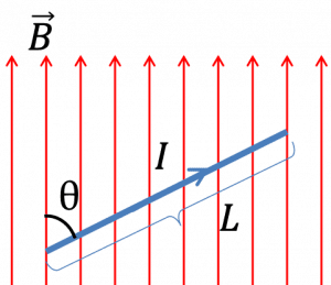
Let us consider a long wire carrying a current I and also consider a point p in the space. You can see the wire below in orange color.

Let us also consider an infinitely small length of the wire dl at a distance r from the point P, see figure below. In the following figure, r is a distance-vector, making an angle θ with the direction of current in the infinitesimal portion of the wire.

If you try to visualize this diagram, then you will see that the magnetic field density at point P due to that infinitesimal length dl of the wire is directly proportional to the current flowing in this wire. This means, the higher the electric current in the wire, the higher the magnetic field density at the point P.

This is not only a work of visualisation. You can do it practical. Take a magnetic compass and place it near to a current carrying wire and see the deflection of magnetic needle at different magnitude of electric current in the wire. You will see that for higher current it show strong deflection and for low current it deflects least.

As the current flowing through the infinitesimal length of wire is the same as the current carried by the whole wire itself, then we can write as-
$$dB\propto I$$
It is also very obvious to think that the magnetic field density at the point P due to that infinitesimal length dl of wire is inversely proportional to the square of the distance from point P to the center of dl. So, mathematically we can also write this as-
$$dB\propto \frac{1}{r^2}$$
And last thing, the magnetic field density at the point P due to that infinitesimal portion of the wire is also directly proportional to the actual length of the infinitesimal length dl of the wire.

And as we know that θ is the angle between the distance vector r and the direction of current through this infinitesimal portion of the wire, then the component of dl directly facing perpendicular to the point P is given as dlsinθ.
$$hence\;dB\propto Idlsin\theta$$
Now, combining all these three above statements, we get-
$$dB\propto \frac{Idlsin\theta}{r^2}$$
This is a basic mathematical statement of Biot-Savart Law.
Now substitute the value of proportionality constant k (which we have discussed at the beginning of the article) in the below equation, then we get-
$$dB= k\frac{Idlsin\theta}{r^2}$$
$$\implies\;dB= \frac{\mu_0 \mu_r}{4\pi} \frac{Idlsin\theta}{r^2}$$
This is the same formula where did we want to reach. So this is the derivation of the Biot-Savart Law.

DIFFERENT EQUATIONS OF BIOT-SAVART LAW

BIOT-SAVART LAW IN THE FORM OF ELECTRIC CURRENT (CLOSED CURVE/WIRE)

The formula which we have derived above is the Biot-Savart Law in the form of electric current. But above formula is not in vector form. In this section, we will see Biot-Savart Law in vector form having current element Idl.

The Biot–Savart is a law which is used to measure the resultant magnetic field B at position r in 3 dimensional-space, which is generated by a wire having current I. 

This law (Biot-Savart Law) is a physical example of a line integral and it is being calculated over the path C in which the electric currents flow (e.g. the wire). The equation in SI units is-
$${\displaystyle \mathbf {B} (\mathbf {r} )={\frac {\mu _{0}}{4\pi }}\int _{C}{\frac {I\,d{\boldsymbol {\ell }}\times \mathbf {r’} }{|\mathbf {r’} |^{3}}}}$$

Where

• ${\displaystyle d{\boldsymbol {\ell }}}$ is a vector along the path ${\displaystyle C}$ whose magnitude is the length of the differential element of the wire in the direction of conventional current.
• ${\displaystyle {\boldsymbol {\ell }}}$ is a point on path ${\displaystyle C}$.
• ${\displaystyle \mathbf {r’} =\mathbf {r} -{\boldsymbol {\ell }}}$ is the full displacement vector from the wire element $({\displaystyle d{\boldsymbol {\ell }}})$ at point ${\displaystyle {\boldsymbol {\ell }}}$ to the point where magnetic field is to be calculated i.e $({\displaystyle \mathbf {r}})$
• And μ0 is the magnetic constant.

Alternatively, it is given as:

$${\displaystyle \mathbf {B} (\mathbf {r} )={\frac {\mu _{0}}{4\pi }}\int _{C}{\frac {I\,d{\boldsymbol {\ell }}\times \mathbf {{\hat {r}}’} }{|\mathbf {r’} |^{2}}}}$$ where ${\displaystyle \mathbf {{\hat {r}}’}}$ is the unit vector of ${\displaystyle \mathbf {r’} }$.

The integral is usually used around the closed curve, where stationary electric currents can only flow around closed paths when they are bounded. However, this law can also be applied to find the value of the magnetic field of infinitely long wires.

Until 20 May 2019, this concept was used to define the SI unit of electric current i.e Ampere.

To apply this equation, Arbitrarily choose a point in space where the magnetic field is to be calculated $({\displaystyle \mathbf {r} })$. Holding that point fixed, the line integral over the path of the electric current is calculated to find the total magnetic field at that point.

The application of the Biot-Savart Law implicitly relies that it follows the superposition principle for the magnetic field, i.e. magnetic field at the point P is the vector sum of the magnetic field created by each of the infinitesimal section of the wire individually.

Biot-Savart Law is usually used to find the magnetic field at the point which is placed arbitrarily at any point in the space.

But there is also a 2D version of this law, it is used when the sources are invariant in one direction. In general, the current need not flow only in a plane normal to the invariant direction and it is given by ${\displaystyle \mathbf {J} }$ (current density). In this case, the resultant formula is given as:
\begin{align*}
\mathbf{B}(\mathbf{r})&=\frac{\mu_0}{2\pi}\int_{C}\frac{(\mathbf{J}d{\ell})\times \mathbf{r}’}{|\mathbf{r}’|}\\
&=\displaystyle{\frac{\mu_0}{2\pi}\int_{C}(\mathbf{J}d{\ell})\times \mathbf{\hat{r}}’}
\end{align*}

BIOT-SAVART LAW IN THE FORM OF ELECTRIC CURRENT DENSITY (THROUGHOUT THE CONDUCTOR VOLUME)

Above formula of Biot-Savart Law work well when the current is running through an infinitely-narrow wire. But if the wire has some thickness, then the proper formulation of the Biot–Savart law in SI unit is given as-

$${\displaystyle \mathbf {B} (\mathbf {r} )={\frac {\mu _{0}}{4\pi }}\iiint _{V}\ {\frac {(\mathbf {J} \,dV)\times \mathbf {r} ‘}{|\mathbf {r} ‘|^{3}}}}$$

Where

• ${\displaystyle \mathbf {r’} }$ is the vector from dV to the observation point ${\displaystyle \mathbf {r} }$
• ${\displaystyle dV}$ is the volume wire element
• And ${\displaystyle \mathbf {J} }$ is the current density vector in that volume.

In terms of unit vector ${\displaystyle \mathbf {{\hat {r}}’}}$, it is given as-

$${\displaystyle \mathbf {B} (\mathbf {r} )={\frac {\mu _{0}}{4\pi }}\iiint _{V}\ dV{\frac {\mathbf {J} \times \mathbf {{\hat {r}}’} }{|\mathbf {r} ‘|^{2}}}}$$

BIOT-SAVART LAW IN THE FORM OF CONSTANT UNIFORM CURRENT

In the form of special uniform constant current, the magnetic field $\displaystyle{\mathbf{B}}$, is given as-

$${\displaystyle \mathbf {B} (\mathbf {r} )={\frac {\mu _{0}}{4\pi }}I\int _{C}{\frac {d{\boldsymbol {\ell }}\times \mathbf {r’} }{|\mathbf {r’} |^{3}}}}$$

Here, you can see that current is taken out of the integral because it is taken as constant.

BIOT-SAVART LAW IN THE FORM OF CONSTANT VELOCITY (POINT CHARGE IN CONSTANT VELOCITY)

Consider a point charged particle q, which is moving at a constant velocity v, then the Maxwell’s equations give the following equations for the electric field and magnetic field
\begin{align*}
\mathbf {E} &={\frac {q}{4\pi \epsilon _{0}}}{\frac {1-{\frac {v^{2}}{c^{2}}}}{\left(1-{\frac {v^{2}}{c^{2}}}\sin ^{2}\theta \right)^{\frac {3}{2}}}}{\frac {\mathbf {{\hat {r}}’} }{|\mathbf {r} ‘|^{2}}}\\
\mathbf {H} &=\mathbf {v} \times \mathbf {D} \\
\mathbf {B} &={\frac {1}{c^{2}}}\mathbf {v} \times \mathbf {E} \end{align*}
where

• ${\displaystyle \mathbf {\hat {r}} ‘}$ is the unit vector pointing from the non-retarded current position of the charge particle to the point at which magnetic field is being calculated.
• And θ is the angle between ${\displaystyle \mathbf {v} }$ and ${\displaystyle \mathbf {r} ‘}$.

If v² is very very less than c² i.e v² \begin{align*}
\mathbf{E}&=\frac{1}{4\pi\varepsilon_0}\frac{\mathbf{\hat{r}}’}{|\mathbf{r}’|^2}\\
\mathbf{E}&=\frac{\mu_0 q}{4\pi}\mathbf{v}\frac{\mathbf{\hat{r}}’}{|\mathbf{r}’|^2}
\end{align*}

These two equations are first derived by the physicist Oliver Heaviside in the year 1888. The equation of the magnetic field $\mathbf{B}$ is sometimes called Biot-Savart Law for a point charge because its close resemblance to the standard version of Biot–Savart law.

However, this language is very misleading that Biot-Savart Law is only applicable for steady currents but the point charge which is moving in free space does not constitute a steady current.

APPLICATIONS OF BIOT-SAVART LAW

Here are listed some applications of Biot-Savart Law-

• The Biot–Savart law can be used in the calculation of magnetic responses at the atomic or molecular level, e.g. chemical shieldings or magnetic susceptibilities, but it should be provided that the current density can be obtained from a quantum mechanical calculation.
• The Biot–Savart law can be also used in aerodynamic theory to calculate the velocity induced by vortex lines.
• It is used to find the magnetic field at a point due to the infinite length of wire.
• It is used to find the magnetic field at a point due to the finite length of the wire.
• It is used to find the magnetic field at a point on the axis passing through the center of the uniform circular current loop.

So this is all about Biot-Savart Law. Stay tuned with Laws Of Nature for more useful and interesting content.